by R. Grothmann
We demonstrate a method be Vanderbei and other authors from 1985-1986 for optimization. There is an implemenation of this method in Euler, which may be useful.
First, we demonstrate inner methods for the example
![]()
![]()
The solution is [3,0,0].
>shortformat; A=[1,1,1]; b=[3]; c=[1,2,3]; x=[1;1;1];
If we start with this x, we get the target value 6.
>c.x
6
Inner methods proceed from x>0 to x>0 using a direction of descent. To find such a direction, we project c to the kernel of A.
First we project c to the image of A', which is perpendicular to the kernel of A.
>y=fit(A',c')
2
In our case, a Gram-Schmidt method can be used.
>(A.c')/(A.A')
2
Now we find the projection to
![]()
>v=c'-A'.y
       -1
        0
        1
We can walk in this direction, until we meet the boundary. Instead we walk only half the way, and stay within the positive quadrant.
>xnew=x-v/2
      1.5
        1
      0.5
The new value is better. Remember, that we minimize!
>c.xnew
5
For the next step, we use the transformation matrix.
This yields an equivalent problem.
![]()
![]()
The trick is that x is now the vector (1,1,1), which is central in the positive quadrant, and promises a quick descent.
>x=xnew; d=x'; tA=A*d; tc=d*c;
We do the same stuff as above in the equivalent problem.
>y=fit(tA',tc');
We get a direction of descent.
>v=tc'-tA'.y
-0.642857
 0.571429
 0.785714
We can go as far as the following value.
>lambda=max(1/v')
1.75
But we go only half that far. Note that we are walking away from the (1,1,1) vector.
>txnew=1-lambda*v/2
   1.5625
      0.5
   0.3125
Transform back.
>xnew=txnew*d'
  2.34375
      0.5
  0.15625
The value is indeed smaller.
>c.txnew
3.5
This process is called affine scaling.
We load the file with the function. It is not yet part of the Euler core.
>load affinescaling;
Here are the details of the implementation.
>type affinescaling
function affinescaling (A: real, b: column real, c: vector real,  ..
gamma: number positive, x: none column real, history, infinite ..
)

## Default for gamma : 0.9
## Default for x : none
## Default for history : 0
## Default for infinite : 4.5036e+011

    n=cols(A);
    if x==none then
        u=b-sum(A);
        A=A|u;
        x=ones(cols(A),1);
        c=c|infinite;
    endif;
    z=c.x;
    if history then X=x; endif;
    repeat
        d=ones(1,cols(A));
        d=x';
        tA=A*d; tc=c*d;
        y=fit(tA',tc');
        v=tc'-tA'.y;
        while !all(v~=0);
        if all(v<=0) then
            error("Problem unbounded");
        endif;
        i=nonzeros(v>0);
        lambda=gamma/max(v[i]');
        tx=x/d'-lambda*v;
        x=d'*tx;
        znew=c.x;
        if history then X=X|x; endif;
        while znew<z;
        z=znew;
    end
    if history then return {x[1:n],X[1:n]};
    else return x[1:n];
    endif;
endfunction
>{xopt,X}=affinescaling(A,b,c,gamma=0.5,x=[1,1,1]',>history); xopt,
        3
        0
        0
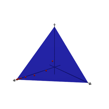
We can plot the points in 3D using Povray. This works only, if Povray is installed and its "bin" directory in the environment variable PATH.
>load povray;
>povstart(distance=9,center=[0,0,1],angle=140°);
>loop 1 to 8; writeln(povpoint(X[:,#]',povlook(red),0.05)); end;
>writeAxes(-0.5,3,-0.5,3,-0.5,3);
>writeln(povplane([1,1,1],3,povlook(blue,0.5),povbox([0,0,0],[4,4,4],look="")));
>povend();
As a second simple example, we demonstrate
![]()
![]()
This writes as.
>A=[1,1;4,5]|id(2)
        1         1         1         0
        4         5         0         1
>b=[1000;4500]
     1000
     4500
>c=-[5,6,0,0]
[-5, -6, 0, 0]
The Simplex method has no problems at all.
>simplex(A,b,c,eq=0,>min,>check)
      500
      500
        0
        0
The algorithm works too. The result is only an approximation, however. We could start there to find an nearby corner.
>affinescaling(A,b,c)
  499.989
   500.01
        0
        0
Another example is
![]()
![]()
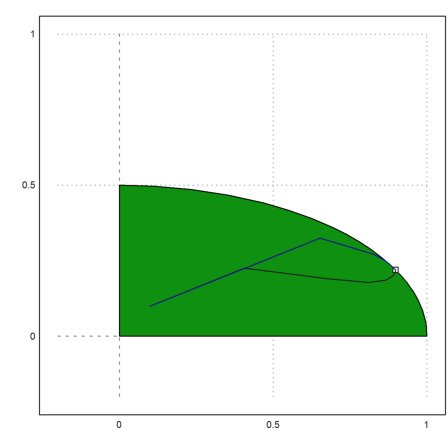
The angle runs from 0 to 90 degrees. The admissible set is an ellipse.
>phi=linspace(0,pi/2,50)'; A=cos(phi)|2*sin(phi);
>b=ones(rows(A),1);
>c=[1,1];
Using the simplex method.
>xopt=simplex(A,b,c,>max,>check)
 0.898138
 0.219997
Let us plot the feasible set.
>P=feasibleArea(A,b);
>plot2d(P[1],P[2],a=-0.2,b=1,c=-0.2,d=1,>filled);
>plot2d(xopt[1],xopt[2],>points,>add):

Now we fill with slack variables, and use affine scaling.
>tA=A|id(rows(A));
>tc=-c|zeros(1,rows(A));
We choose an inner point by computing all slack variables.
>x=[0.1,0.1]'; x=x_(b-A.x);
>{xopt,X}=affinescaling(tA,b,tc,0.5,x,>history);
We kill the slack variables, and get the same result.
>xopt[1:2]
 0.898138
 0.219997
But the path the algorithm takes is quite different from the simplex method, which goes around the vertices at the boundary.
>plot2d(X[1],X[2],>add):

Here is the number of steps the algorithm took.
>cols(X)
29
With gamma=0.9, the algorithm takes less steps.
>{xopt,X}=affinescaling(tA,b,tc,0.9,x,>history);
>cols(X)
17
>plot2d(X[1],X[2],color=blue,>add):
It is better to use the dual problem here, since the matrix is only 2x51.
>lopt=affinescaling(A',c',b');
We search for the two active lambdas.
>{xs,js}=sort(-lopt); j=js[1:cols(A)]
       16
       15
Then we solve for the primal solution.
>x=A[j]\b[j]
 0.898138
 0.219997